Into the INFERNO: parameter estimation under uncertainty - Part 3
In this series of posts, we'll be looking at one of the most common problems in high-energy physics; that of estimating some parameter of interest. In this third post we'll finally start looking in to the INFERNO paper example, and showing how the typical approaches used in HEP aren't always optimal.


Welcome back to the third part of this blog-post series. In case you missed it, the first and second parts may be found here and here. Last time we finished laying the necessary groundwork for parameter estimation, and in this post we'll look at the example presented in the INFERNO paper, and demonstrate how the typical approach in HEP would go about solving it.
For the rest of this blog-post series, we'll be using a PyTorch implementation of INFERNO which I've put together, but I'll do my best to show the relevant code, and explain what each component does. The package can be installed using:
!pip install pytorch_inferno==0.0.1
Docs are located here and the Github repo is here. I'm installing v0.0.1 here, since it was what I used when writing this post, but for your own work, you should grab the latest version.
As an additional note, these blog posts are fully runnable as Jupyter notebooks. You can either download them, or click the Google Colab badge at the top to follow along!
Similar to our examples in the previous two posts, the paper considers a toy example in which two classes of process (signal and background) contribute to an observed count. The count density is defined using three arbitrary features, $\bar{x}=(x_0,x_1,x_2)$, and differences in the probability distributions functions (PDFs) of the two classes can be exploited in order to improve the precision of the parameter of interest, $\mu$, which is the signal strength scaling the contributions of the signal process: $N_o=\mu s + b$, where $N_o$ is the observed count and $s$ and $b$ are the expected contributions from the signal and background processes.
The PDFs of the two classes are specified using a 2D Gaussian distribution and an exponential distribution: $$f_b(\bar{x}) = \mathcal{N}\left((x_0,x_1)\,|\,(2,0),\begin{bmatrix}5&0\\0&9\end{bmatrix}\right)\mathrm{Exp}(x_2\,|\,3)$$ $$f_s(\bar{x}) = \mathcal{N}\left((x_0,x_1)\,|\,(0,0),\begin{bmatrix}1&0\\0&1\end{bmatrix}\right)\mathrm{Exp}(x_2\,|\,2)$$
N.B. Eq.15 in the paper states the means of the signal Gaussian are $(1,1)$, however the code on which the results are derived used $(0,0)$.
In the package, this is implemented as:
class _PaperData():
    r'''Callable class generating pseudodata from Inferno paper'''
    def __init__(self, mu:List[float], conv:List[List[float]], r:float, l:float):
        store_attr(but=['mu', 'r'])
        self.r = np.array([r,0])
        self.mu = np.array(mu)

    def sample(self, n:int) -> np.ndarray:
        return np.hstack((np.random.multivariate_normal(self.mu+self.r, self.conv, n),
                          np.random.exponential(1/self.l, size=n)[:,None]))

    def __call__(self, n:int) -> np.ndarray: return self.sample(n)
r is a nuisance parameter which can affect the mean of the Gaussian, but we'll get to that later on.
from pytorch_inferno.pseudodata import _PaperData
_PaperData(mu=[0,0], conv=[[1,0],[0,1]], r=0, l=2).sample(2)
Sampling two points, returns the values of the three features for both points. Let's generate samples for signal and background, and plot out the features:
%%capture --no-display
from pytorch_inferno.pseudodata import PseudoData, paper_bkg, paper_sig
import seaborn as sns
n=1000
df = PseudoData(paper_sig, 1).get_df(n).append(PseudoData(paper_bkg, 0).get_df(n), ignore_index=True)
sns.pairplot(df, hue='gen_target', vars=[f for f in df.columns if f != 'gen_target'])

From the distributions above we can see that the signal (1-orange) overlaps considerably with the background (0-blue), which no particular feature offering good separation power; the features as they stand are unsuitable for inferring $\mu$ via binning. $x_1$ perhaps could be used, since the background displays a greater spread than the signal, however we can hope to do better.
As stated last time, what we want is a single feature in which the classes of signal and background are most linearly separable. This has to be a function of the observed features $\bar{x}$: $$f(\bar{x})=y,$$ where $y=0$ for background and $y=1$ for signal. I.e. $f$ maps $\bar{x}$ into a space in which the two processes are completely distinct. Unfortunately, such as function is not always achievable given the information available in $\bar{x}$. Instead we can attempt to approximate $f$ with a parameterisation: $$f_\theta(\bar{x})=\hat{y}\approx y,$$ Since $f_\theta$ is only an approximation, the resulting predictions $\hat{y}$ will be a continuous variable in which (hopefully) background data will be clustered close to zero and signal clustered close to one.
Depending on any domain knowledge available, suitable (monotonically related) forms of $f_\theta$ may be available in the form of high-level features: E.g. when searching for a Higgs boson decaying to a pair of tau leptons, the invariant mass of the taus should form a peak around 125 GeV for signal whereas background should not form a peak. Such a high-level feature can then either be transformed into the range [0,1] or just binned for inference directly.
A better approach (usually), especially when domain theory cannot help, however is to learn the form of $f_\theta$ from example data using a sufficiently flexible model by optimising the parameters $\theta$ such that: $$\theta=\arg\min_\theta[L(y,f_\theta(\bar{x})],$$ where the loss function $L$ quantifies the difference between the predictions of the model $f_\theta(\bar{x})$ and the targets $y$.
Common forms of $f_\theta(\bar{x})$ in HEP are Boosted Decision Trees and now more recently (deep) neural networks ((D)NNs. Eventually I'll write a new series on DNNs, but for now I can point you to my old series here. I'll proceed assuming a basic understanding of DNNs, I'm afraid, so as not to go beyond scope.
Let's train a DNN as a binary classifier to predict whether data belongs to signal or background. The pytorch_inferno package includes a basic boilerplate code for yielding data and training DNNs.
As per the paper, we'll use a network with three hidden layers network and ReLU activations to map the three input features to a single output with a sigmoid activation.
from pytorch_inferno.utils import init_net
from torch import nn
net = nn.Sequential(nn.Linear(3,100),  nn.ReLU(),
                    nn.Linear(100,100),nn.ReLU(),
                    nn.Linear(100,1),  nn.Sigmoid())
init_net(net)  # Initialise weights and biases
The ModelWrapper class then provides support for training the network, and saving, loading, and predicting.
from pytorch_inferno.model_wrapper import ModelWrapper
model = ModelWrapper(net)
A training and testing dataset can be generated and wrapped in a class to yield mini-batches.
from pytorch_inferno.data import get_paper_data
data, test = get_paper_data(n=200000, bs=32, n_test=1000000)
Now let's train the model. In contrast to the paper, we'll use ADAM for optimisation, at a slightly higher learning rate, to save time. We'll also avoid overtraining by saving when the model improves using callbacks. The Loss is binary cross-entropy, since we want to train a binary classifier.
from fastcore.all import partialler
from torch import optim
from pytorch_inferno.callback import LossTracker, SaveBest, EarlyStopping
model.fit(200, data=data, opt=partialler(optim.Adam,lr=8e-4), loss=nn.BCELoss(),
          cbs=[LossTracker(),SaveBest('weights/best_bce.h5'),EarlyStopping(5)])
Having trained the model, we can now check the predictions on the test set
preds = model._predict_dl(test)
import pandas as pd
df = pd.DataFrame({'pred':preds.squeeze()})
df['gen_target'] = test.dataset.y
df.head()
from pytorch_inferno.plotting import plot_preds
plot_preds(df)

From the above plot, we can see that the model was able to maps both classes towards their target values. It also shows good agreement with Fig. 3a in the paper.
Now that we have learnt a feature (the DNN predictions) in which the signal and background a highly separated, we're now in a position to estimate our parameter of interest by binning the PDFs of signal and background, as per the last post.
Similar to the paper, we'll bin the predictions in 10 bins of equal size:
from pytorch_inferno.inference import bin_preds
import numpy as np
bin_preds(df, np.linspace(0,1,11))  # Bins each prediction

df.head()
Now we want to get the PDFs for signal and background
from pytorch_inferno.inference import get_shape
f_s,f_b = get_shape(df,targ=1),get_shape(df,targ=0)  # Gets normalised shape for each class
f_s,f_b
In this example (and generally in HEP) we use simulated data to estimate the PDFs of signal and background. The expected yields (overall normalisation) are separate parameters. This is to say that although we trained our model on 200,000 datapoints, and estimated the PDFs on 1,000,000 data points, these sample sizes need not have any relationship to the expected yields of signal and background; for the paper example, the background yield is 1000, and the signal yield is our parameter of interest, $\mu=50$.
At this stage of a proper HEP analysis, we would still be optimising our analysis and so will not have access to the observed data. Instead, as mentioned last time, we can check expected performance by computing the Asimov dataset; the expected yield per bin, where any parameters are at their expected yield. I.e., the Asmiov yield in bin i will be: $$N_a=50\cdot f_{s,i}+1000\cdot f_{b,i}$$
asimov = (50*f_s)+(1000*f_b)
asimov, asimov.sum()
Now we can compute the negative loglikelihood for a range of $\mu$ values, as usual
import torch
n = 1050
mu = torch.linspace(20,80,61)
nll = -torch.distributions.Poisson((mu[:,None]*f_s)+(1000*f_b)).log_prob(asimov).sum(1)
nll
from pytorch_inferno.plotting import plot_likelihood
plot_likelihood(nll-nll.min())

Comparing the width to Tab.2 in the paper (NN classifier, Benchmark 0 = 14.99), our value seems to be in good agreement!
There are two ways in which nuisance parameters can affect our measurement: 1) the nuisance parameter leads to a shift in the PDF of a class, but the overall normalisation stays the same; 2) the PDF stays the same, but the normalisation changes. Both of these types of nuisances can be constrained by auxiliary measurements, as described in part-1.
The paper considers a range of benchmarks for how the presence of different nuisances can affect the precision of the measurement:
- The mean of the Gaussian distribution of the background is allowed to shift in one dimension by an amount $r$
- In addition to 1) the rate of the Exponential distribution, $\lambda$, of the background is allowed to change
- Similar to 2), except $r$ and $\lambda$ are constrained by auxiliary measurements
- Similar to 3), except now the overall background rate, $b$ is allowed to shift and is constrained by an auxiliary measurement
The uncertainty of $r$ and $\lambda$ leads to changes in the input features of our model, and so leads to changes in the PDF of the background distribution of the inference feature. When attempting to minimise the negative log-likelihood, by optimising the nuisance parameters, these shifts must be accounted for: if the $r$ shift is +0.2, then all of the $x_0$ features for the background are shifted by +0.2, which means that the predictions of the DNN will also change in some more complex way. Similarly, if $\lambda$ is increased by 0.5, then the whole of $x_3$ for background are multiplied by a factor $3.5/3$.
We are lucky in this example, that the analytic effects on the input features of these two nuisances can be computed; sometimes this is not the case. In HEP, simulated data are generated by stochastic modelling, and the exact effect on a given variable of say jet energy scale or tau ID cannot be analytically derived. The approach, then, is to generate additional datasets in which the values affected by the systematics are moved up and down according to their uncertainty (e.g. one would have a nominal dataset, and then JES_UP and JES_DOWN datasets in which the energy scale is shift up/down by 1-sigma). These additional datasets are then also fed through the DNN, in order to arrive at up/down shifts in the PDFs. Since the analytical effects on the input features in our example systematics are known, we can simply adjust the existing dataset and pass it through our model.
Let's now compute all the shifts in the background PDF. Following the paper, $r$ is shifted by $\pm0.2$, and $\lambda$ by $\pm0.5$. Remember that these shifts only affect the background process. get_paper_syst_shapes will shift the data, recompute the new model predictions, and then compute the new PDF for background
from pytorch_inferno.inference import get_paper_syst_shapes
bkg = test.dataset.x[test.dataset.y.squeeze() == 0]  # Select the background test data
b_shapes = get_paper_syst_shapes(bkg, df, model=model, bins=np.linspace(0,1,11))
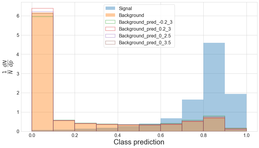
The function also saves the new predicted bin to the DataFrame, allowing us to see how the background shifts compared to the nominal prediction.
plot_preds(df, pred_names=['pred', 'pred_-0.2_3', 'pred_0.2_3', 'pred_0_2.5', 'pred_0_3.5'])

So we can see that the changes in the nuisance parameters really do result in shifts in the background PDF. In b_shapes we have a a dictionary of the nominal, up, and down shifts according to changes in $r$ and $\lambda$.
b_shapes
These shifts, however, are discrete and our optimisation of the values of $r$ and $\lambda$ needs to happen in a continuous manner, but generating new simulated data at the desired nuisance values is too time consuming. Instead we can interpolate between the systematic shifts and the nominal values in each bin in order to estimate the expected shape of the PDF for proposed values of the nuisances. Additionally, such shifts need to happen in a differentiable manner, so that we can optimise the nuisance values using the Newtonian method, as per part-1.
The interp_shape function performs a quadratic interpolation between up/down shifts and the nominal value, and a linear extrapolation outside the range of up/down shifts, and does so in a way that allows the resulting values to be differentiated w.r.t. the nuisance parameters. For example in bin zero, we can plot (in red) the computed PDF values at up (1.0), nominal (0.0), and down (-1.0), and also then plot the results of the interpolation and extrapolation for shifts in $r$ (blue scatter). The corresponding PDF value is shown in the y-axis.
from pytorch_inferno.inference import interp_shape
from torch import Tensor
import matplotlib.pyplot as plt

i = 0
d = b_shapes['f_b_dw'][0][i]
n = b_shapes['f_b_nom'][i]
u = b_shapes['f_b_up'][0][i]
interp = []
rs = np.linspace(-2,2)
for r in rs: interp.append(interp_shape(Tensor((r,0))[None,:], **b_shapes)[0][i].data.item())
plt.scatter(rs, interp)
plt.plot([-1,0,1],[d,n,u], label=i, color='r')

Let's now evaluate our trained model under Benchmark 2, in which both $r$ and $\lambda$ are completely free. The process of minimising the NLL at each value of $\mu$ is now slightly more complicated than before since we now have multiple nuisances, and so need to compute the full Jacobian and Hessian matrices (as warned in part-1).
Unfortunately here either my PyTorch skills fail me, or PyTorch lacks sufficient flexibility, but I haven't yet managed to perform these calculations in a batch-wise manner. Meaning that the NLL optimsation must be done in series for every value of $\mu$, rather than in parallel as before. I think the problem is that PyTorch is overly secure and refuses to compute gradients when not all variables are present, even if they aren't necessary to compute the gradients. So if anyone has any ideas, please let me know!
Anyway, let's use the calc_profile function to minimise the nuisances for a range of signal strengths and return the NLL
%%capture --no-display
from pytorch_inferno.inference import calc_profile
profiler = partialler(calc_profile, f_s=f_s, n=1050, mu_scan=torch.linspace(20,80,61), true_mu=50, n_steps=100)
nll = profiler(**b_shapes).cpu().detach()
plot_likelihood(nll-nll.min())

Right, so the uncertainty has gone way up! What a shame.
We can slightly improve things by including auxiliary measurements on $r$ and $\lambda$. Benchmark 3 in the paper considers constraints as Gaussian distributions with standard deviations equal to 2, so let's include those in the NLL minimisation.
N.B. in contrast to the paper and paper code, in the implementation here, systematics are treated as new parameters perturbing existing parameters from their nominal values, rather than being the existing parameters themselves.
%%capture --no-display
alpha_aux = [torch.distributions.Normal(0,2), torch.distributions.Normal(0,2)]
nll = profiler(alpha_aux=alpha_aux, **b_shapes).cpu().detach()
plot_likelihood(nll-nll.min())

The constraints restore some sensitivity, but we're still doing much worse than before, when we didn't consider the nuisance parameters.
The second way that nuisances can affect the measurement, is by globally rescaling the background contributions (i.e. letting $b$ float when minimising the NLL). As we saw in part-1 these kinds of nuisances really need to be constrained, however with the binned approach, we do have some slight resilience to them, unlike before where they completely killed our sensitivity.
%%capture --no-display
nll = profiler(alpha_aux=alpha_aux, float_b=True, b_aux=torch.distributions.Normal(1000,100), **b_shapes).cpu().detach()
plot_likelihood(nll-nll.min())

Ouch, that really doesn't look good!
So what we've seen here is that by using a neural network we can map a set of weakly discriminating features down into a single powerful feature, and use it for statistical inference of parameters in our model. When applicable, this is the typical approach now in contemporary HEP, (and has been used to get some really great results over the years!).
Unfortunately, what we've also seen is that the presence of nuisance parameters (systematic uncertainties) can really spoil the performance of the measurement. Both by altering the input features, leading to flexibility in the shape of the inference variable, and by adjusting the overall normalisation of different processes contributing to the observed data (or its Asimov expectation).
The way in which we map the weak features down to the single, strong feature, and the way that we bin the resulting distribution, should ideally be done in a manner which accounts for the effects of the nuisance parameters that will later be included in the parameter estimation. This is precisely what the INFERNO method sets out to accomplish, and in the next post, we shall begin looking at how this can be achieved.