Into the INFERNO: parameter estimation under uncertainty - Part I
In this series of posts, we'll be looking at one of the most common problems in high-energy physics; that of estimating some parameter of interest. In this first post we'll look at the statistical framework for making measurements, and seeing how these can be spoilt once we introduce uncertainties on other parameters in our measurement.


In this series of posts, we'll be looking at one of the most common problems in high-energy physics; that of estimating some parameter of interest. In this first post we'll look at the statistical framework for making measurements, and seeing how these can be spoilt once we introduce uncertainties on other parameters in our measurement.
This situation can be improved, however, though an approach called Inference Aware Neural Optimisation (INFERNO) developed by Pablo de Castro Manzano and Tommaso Dorigo, and over the next few posts I'll be breaking down the paper and explaining the approach in runnable code. Accompanying this series will be a PyTorch implementation of their method, but for this initial post we don't need it.
Whilst this method is potentially applicable to a wide range of problems, I'm a particle physicist, and so will be describing the problem primarily from that point of view.
- 2020/12/14: Corrected plotting function to compute nll widths at 0.5 (previously was 1)
Commonly in high-energy particle physics, such as the work performed at the Large Hadron Collider at CERN, we want to estimate some parameter of our theoretical model. This could perhaps be rate at which some new process contributes to the data we collect. If a given region of our observed data contains $N_o$ data points (events) and processes already included in our model (referred to as background) contribute $N_b$ events, then one might say that any surplus event count is due to some new process which is not included in our model (signal):
$$N_s=N_o-N_b.$$
The problem is that different process contribute as a random Poisson process; we can compute the mean rate via Monte Carlo simulation but we never know the exact contributions of each process in the observed data, i.e. we instead are comparing the observed count with the expected process contributions, $\left<N_s\right>+\left<N_b\right>$. For ease of writing, I'll refer to these expected counts as $s$ and $b$.
For the problem of evaluating the presence of signal in our data, it is useful to parameterise the expected count as:
$$n=\mu s+b,$$
where $\mu$ is a coefficient controlling the level of signal contribution. $\mu=0$ would therefore mean no signal contribution. This signal strength is our parameter of interest; we want to construct an experiment that allows us to measure this parameter as precisely as possible.
Unfortunately, the problem can be further complicated by the fact that our theoretical model may not be fully specified: we may only know the mean value of the mean contribution of background, i.e. the model for the background contains unknown parameters and we've simply assumed values for them based on expectation or prior measurements.
These nuisance parameters ($\theta$) can affect the expected background contribution, making the signal contribution more difficult to estimate:
$$n(\mu,\theta)=\mu s+b(\theta).$$
Our ultimate aim is to adjust our model so that it describes the observed data as well as possible. This means adjusting the parameters of the model in order to improve its goodness-of-fit through a maximum likelihood fit. Our likelihood function for these uncertain Possion contributions to an observed count $N_o$ is:
$$L(\mu,\theta)=\frac{(\mu s+b(\theta))^{N_o}}{N_o!}e^{\mu s+b(\theta)}$$
The parameters $\mu$ and $\theta$ can then be adjusted in in order to maximise the likelihood, meaning that our best estimate of the parameter of interest is:
$$\hat{\mu} = \arg\max_{\mu,\theta}L(\mu,\theta)$$
The above formulation will give us an estimation of the parameter of interest, $\mu$. However every experiment will give us a measurement of $\mu$. What really matters when constructing the experiment is the associated uncertainty on the resulting measurement of $\mu$.
We can compute the uncertainty on our measurement by testing a range of possible values for $\mu$ and maximising the likelihood at that value by only adjusting the nuisance parameters.
$$\hat{L}(\mu_i,\hat{\theta}) = \max_{\theta}L(\mu_i,\theta)=\max_{\theta}\left[\frac{(\mu_i s+b(\theta))^{N_o}}{N_o!}e^{\mu_i s+b(\theta)}\right]$$
The nuisance parameters compensate for the lack of freedom on $\mu$, allowing the likelihood to be maximised above what would be possible if the nuisance parameters were not present. This effect is illustrated in the figure below:
Whilst the value of $\mu$ which maximises the likelihood remains the same, the presence of nuisances increases the width of the likelihood thereby reducing our experiment's sensitivity to the exact value of $\mu$.
Let's take a quick look at what is really going on here in terms of code. We'll be working in PyTorch since we'll be making use of it's automatic differentiation later on. First we'll import the necessary stuff.
%matplotlib inline
import matplotlib.pyplot as plt
from fastcore.all import is_listy
from typing import List, Optional, Tuple
from scipy.interpolate import InterpolatedUnivariateSpline
import numpy as np

import torch
from torch import Tensor, autograd, distributions
As a semi-abstract example let's say that we observe 1100 events ($n$), and our background model predicts that we should observe an average of 1000 events ($b$). In addition to the background, there is a possible signal process (which may or may not exist), which can contribute an extra $\mu$ number of events.
b = 1000
n = 1100
In this case the best-fit value of $\mu$ is 100, however what also matters is the uncertainty on $\mu$ that our measurement carries. To evaluate this, we first compute the likelihood as a function of $\mu$.
$$L(\mu)=\frac{(\mu+b)^{n}}{n!}e^{\mu+b}$$
For computational reasons:
- We usually compute the natural log of the likelihood (e.g. PyTorch distributions only offer a
log_probmethod) - We rearrange the problem into a minimisation problem, rather than a maximisation one (functional optimisation traditionally deals with the minimisation of some cost function)
All this is to say that rather than maximising the likelihood, we will instead be minimising the negative log-likelihood (nll). So to compute this, first compute the mean of the Poisson distribution ($\mu+b$=t_exp), and then we evaluate the natural log of the probability at the number of observed events $n$.
def compute_nll(mu:Tensor) -> Tensor:
    t_exp = mu+b
    return -torch.distributions.Poisson(t_exp).log_prob(n)
The above function is vectorised, so we can compute the nll of a range of $\mu$ values simultaneously.
mu_range = torch.linspace(0,200)
nlls = compute_nll(mu_range)
Let's plot them out. Notice how the nll reaches a minimum value at 100, and then increases as $\mu$ moves away from 100, indicating that the level of agreement of our model with the observed data is decreasing.
plt.plot(mu_range,nlls)
plt.xlabel('$\mu$')
plt.ylabel('$-\ln L$')
plt.show()

As mentioned earlier, we are most interested in comparing measurements in terms of the width of the likelihood function (uncertainty on $\mu$ measurement). For convenience, let's write a plotting function that shifts the likelihoods to zero (nlls-nlls.min()=$\Delta nll$), and computes the width at $\Delta nll=0.5$, which corresponds to one standard deviation.
def plot_nlls(nlls:List[Tensor], mu_scan:Tensor, labels:Optional[List[str]]=None) -> List[float]:
    if not is_listy(nlls): nlls = [nlls]
    if labels is None: labels = ['' for _ in nlls]
    elif not is_listy(labels): labels = [labels]

    widths = []
    plt.figure(figsize=(16,9))
    plt.plot(mu_scan,[0.5 for _ in mu_scan], linestyle='--', color='black')
    for nll,lbl in zip(nlls,labels):
        dnll = nll-nll.min()  # Shift nll to zero
        roots = InterpolatedUnivariateSpline(mu_scan, dnll-0.5).roots()  # Interpolate to find crossing points at dll=0.5
        if len(roots) < 2: widths.append(np.nan)  # Sometimes the dnll doesn't cross 1
        else:              widths.append((roots[1]-roots[0])/2)  # Compute half the full width (uncertainty on mu)
        plt.plot(mu_range, dnll, label=f'{lbl} Width={widths[-1]:.2f}')
    plt.legend(fontsize=16)
    plt.xlabel('$\mu$', fontsize=24)
    plt.ylabel('$\Delta (-\ln L)$', fontsize=24)
    plt.show()

    return widths
_ = plot_nlls(nlls, mu_range)

Let's now imagine an example in which a nuisance parameter ($\theta$) affects the level of contribution the background process has. I.e. there is some part of the background model which is not fully specified. In this case we must perform a profile fit of this nuisance parameter, when evaluating the likelihood at each value of the parameter of interest, $\mu$.
As before, we will be aiming to minimise the negative log-likelihood:
$$\hat{L}(\mu_i,\hat{\theta}) = \min_{\theta}\left[-\ln\left[\frac{(\mu_i+(1+\theta)b)^{n}}{n!}e^{\mu_i+(1+\theta)b}\right]\right]$$
def compute_nll(mu:Tensor, theta:Tensor) -> Tensor:
    t_exp = mu+((1+theta)*b)
    return -torch.distributions.Poisson(t_exp).log_prob(n)
Now that our computation of the nll includes the background rate uncertainty, we need someway to minimise it by varying the value of the nuisance parameter. Both the authors' Tensorflow 1 implementation and Lukas Layer's Tensorflow 2 version use Newtonian optimisation, so let's go with that.
In this iterative method, $\arg\min_\theta f(\theta)$ can be found via updates to $\theta$ of the form:
$$\theta_{k+1} = \theta_k-\gamma\frac{f'}{f''},$$
where $f'$ is the derivative of $f$ with respect to $\theta$ at the value $\theta_k$, and $f''$ is the derivative of $f'$ with respect to $\theta_k$ (the second derivative). $\gamma$ controls the rate of convergence (similar to a learning rate).
This is where PyTorch's automatic differentiation really becomes useful; we can compute nll, and then differentiate it w.r.t. the nuisance parameter in order to compute the update step for the value of nuisance parameter.
One subtlety in the above form is that when multiple nuisances are involved, they must be updated simultaneously, i.e. $f'$ must be the derivative w.r.t. a vector of nuisance parameters $\bar{\theta}$ (the Jacobian). $f''$ is then a matrix of derivatives of $f'$ w.r.t $\bar{\theta}$ (the Hessian).
Further complication arises when computing $\frac{f'}{f''}$, since the inverse of $f''$ must instead be computed, and multplied to $f'$. Inverting matrices can be computationally difficult, however for a small number of parameters, it should be manageable (this is one reason why such second-order methods aren't used for optimising neural networks).
def optimise_theta(mu:float, n_steps:int=100, lr=0.1) -> Tensor:
    def calc_derivatives(nll:Tensor, theta:Tensor) -> Tuple[Tensor, Tensor]:
        first  = autograd.grad(nll,   theta, torch.ones_like(nll), create_graph=True)[0]
        second = autograd.grad(first, theta, torch.ones_like(first))[0]
        return first, second

    theta = torch.zeros_like(mu, requires_grad=True)  # Initaialise the nuisance to zero
    for i in range(n_steps):  # Newton optimise nuisances
        nll = compute_nll(mu, theta)
        first, second = calc_derivatives(nll, theta)  # Differentiate NLL w.r.t. the nuisance parameter
        step = lr*first/second
        theta = theta-step
    return theta.cpu().detach()  # Return the optimal value of nuisance parameter
Similar to the nll calculation, the function above is vectorised, so we can optimise multiple values of the nuisance parameter simultaneously (and independently).
theta = optimise_theta(mu_range)
nlls_uncertain = compute_nll(mu_range, theta)
Let's plot out this likelihood.
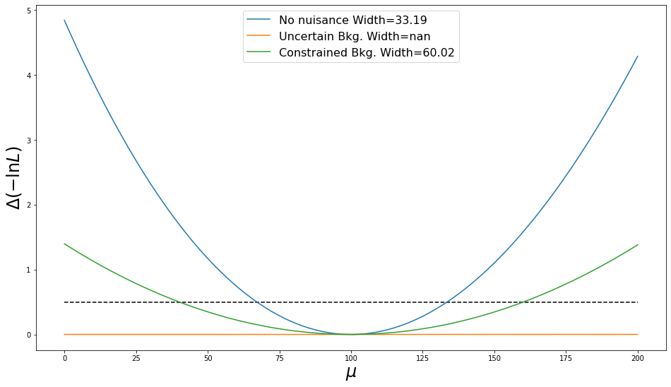
_ = plot_nlls([nlls, nlls_uncertain], mu_range, labels=['No nuisance', 'Uncertain Bkg.'])

Oh no! We've completely lost all sensitivity to the parameter of interest. This is because the nuisance is free to take any value, and so can compensate for the variation in $\mu$ in order to consistently produce an expected count of 1100 events to match the observed data.
In order to avoid situations like the above, other measurements of the background model can be included to help dictate reasonable values of the nuisance parameter (referred to as auxiliary measurements and constraints). Such auxiliary measurements typically come with their own associated uncertainties.
Continuing our example, let's say we already measured the nuisance parameter $\theta$ and arrived at a value of $0\pm0.05$, i.e. the nuisance doesn't appear to affect the background yield, however we're not completely certain. We can include the measurement to constrain the nuisance by assuming it follows a Gaussian distribution, centred at zero with a standard deviation of 0.05.
Whilst $\theta$ is still free to take any value, the likelihood receives a contribution from the auxiliary measurement in the form of a log-Normal evaluated at the proposed value of $\theta$. I.e. if the value of $\theta$ strays far from zero, then the likelihood receives a penalty.
def compute_nll(mu:Tensor, theta:Tensor) -> Tensor:
    t_exp = mu+((1+theta)*b)
    nll = -torch.distributions.Poisson(t_exp).log_prob(n)
    nll -= distributions.Normal(0,0.05).log_prob(theta)  # Subtract the log-probability according to aux measurement
    return nll
theta = optimise_theta(mu_range)
nlls_constrained = compute_nll(mu_range, theta)
_ = plot_nlls([nlls, nlls_uncertain, nlls_constrained], mu_range,
              labels=['No nuisance', 'Uncertain Bkg.', 'Constrained Bkg.'])

So, with our auxiliary measurement of the nuisance parameter, we once again have sensitivity to our parameter of interest. However, the extra flexibility the model has from nuisance parameter means that the measurement is still worse than if the background model were fully specified (larger width).
Here we've begun looking to the statistical framework for estimating a parameter of interest when nuisance parameters are present. However we've so far ignored the methods by which the counts are gained. In the next post we'll look into how measurements can be improved by considering multiple regions of the data-space, and how the typical approaches (in HEP) aren't always optimal once nuisances are included.
Of course, I'd recommend reading through the INFERNO paper. I'll be breaking down the method itself, but the paper gives an in depth discussion about the context, problem, and other work.
For an introduction to the statistical framework used in HEP, I'd recommend (at least Section 2) of Asymptotic formulae for likelihood-based tests of new physics by Glen Cowan, Kyle Cranmer, Eilam Gross, and Ofer Vitells.