Differentiable Programming and MODE
Take-home messages from a recent workshop, and the role of differential optimisation in detector design.
- What is Differentiable Programming?
- Why MODE?
- How does/can differential programming help
- Differential Optimisation in Action
- Conclusion
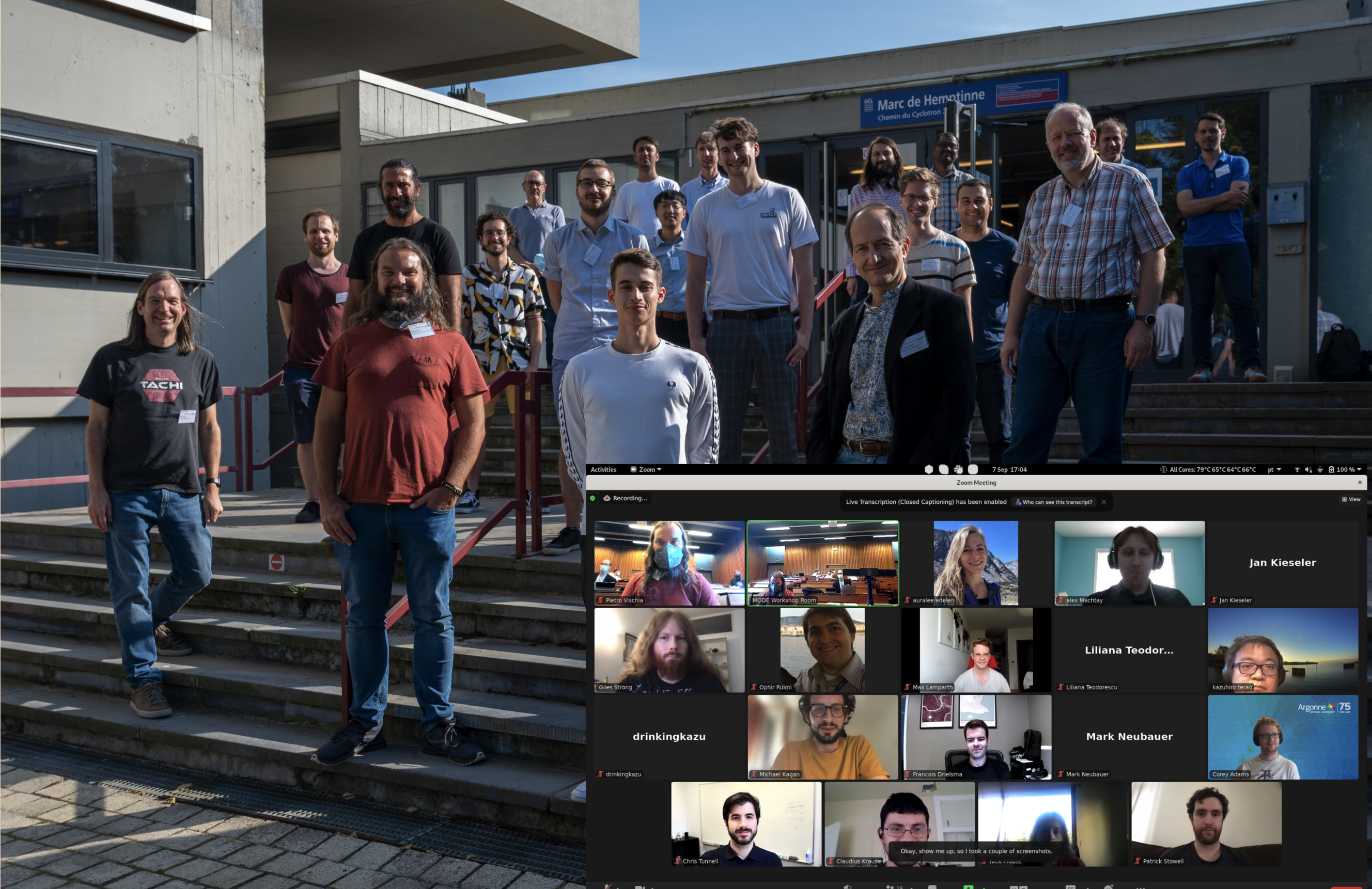
Earlier this week, I had the pleasure to follow a jam-packed meeting of experts from around the world discussing the application of differential programming to the topic of experiment planning and optimisation. This workshop was organised by the MODE collaboration (a new consortium dedicated to Machine-learning Optimized Design of Experiments, of which yours truly is a member), and kindly hosted by UCLouvain, Belgium. Alongside planning sessions for MODE activities, we heard talks on a range of topics, primarily in the domains of computer science and particle physics. I’ll aim to summarise below, the main discussion points.
What is Differentiable Programming?
In his opening lecture, Atılım Güneş Baydin (MODE, University of Oxford), quoted Differentiable Programming (DP) as a generalisation of Deep Learning (DL); a style of software writing in which lines of code are not explicitly written by the developer, but instead the program is composed of differentiable modules (e.g. neural nets, or other, more simple functions). Through the use of automatic differentiation, these modules can be adjusted such that they fulfil their expected role.
Likely, readers will be familiar with how a convolutional neural network (CNN) can be trained to identify cats, dogs, etc. in images, but consider now a system which instead writes out a text description of the image.
One approach would be to train the CNN to output objects and their positions, and then train a text generator to take these objects and positions and write a summary. However the system is limited by the developer’s choice of CNN output, which forces the image representation to be something traditionally understandable by humans.
The “software 2.0” approach is to forfeit some degree of interpretability and allow the CNN to interpret the image into an information-rich latent space representation, and the text-generator to process this representation into words. Whilst we could pre-train both of these blocks in isolation, the full optimisation will involve training both blocks simultaneously, and in so doing reduce the limitations on the system that would otherwise be present if the blocks were kept separate.
In the first approach we solve our task by creating two artificial subtasks and solving those in isolation. We may be able to solve these subtasks optimally, but that doesn’t guarantee that the complete task will be optimally solved. In the second approach, we specify blocks, connect them up, and solve our task directly.
The figure below shows examples of what the two approaches might achieve: in the first approach, the hypothetical developer did not include any possibility to output texture or overall image colour and this limits the output possibilities of the text generator; whereas in the second approach, embeddings for these details could be learnt via the end-to-end training and do not have to be explicitly included.
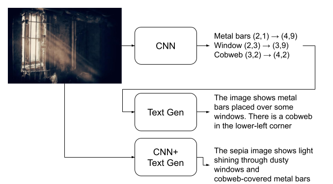 Photo credits: Denny Müller
Why MODE?
The workshop began with an introductory talk from Tommaso Dorigo (MODE, INFN-Padova, CMS), in which he lamented that the design of large-scale scientific instruments, such as particle detectors like those found at CERN, was still very much dominated by the immovable beliefs of an old guard of proficient experts, with well-established (but mathematically unproven) design doctrines.
Three identified weaknesses are:
-
Designs would be created without full consideration of the particle-reconstruction algorithms that will be applied to the detector signals; and with the rise of DL such gaps between design and usage grow even wider.
-
Detector design takes place with limited communication between designers and researchers; there is no quick way to measure the impact a design choice has on the end physics goals of the detector.
-
Human limitations ⇒ design limitations: difficult to design in 3D, therefore create in 2D and stack modules together; design part of the detector, and mirror it, even though not all physical processes are symmetric; unable to consider all possible designs when trying to keep to a budget.
All three of these concerns stem from approaching the problem by splitting the design into subtasks and solving each in isolation. If the aim is to discover di-Higgs production, the detector design process is: design transparent trackers to measure charged particle momenta via magnetic curvature; design dense calorimeters to destroy particles and measure their energy; design sub-detectors to time when particles exit the detector; hope it’s under budget otherwise run studies to see if money can be saved somewhere. Only once a mature design is in place would a few aspects of the design be fine tuned by estimating their effects on the sensitivity to di-Higgs production (see e.g. tables 5.2 and 5.3 of CMS-TDR-020).
As we’ve discussed in the previous section, such isolation of tasks limits optimisation to the study of proxy objectives, which may only be loosely indicative of the desired goal. Dorigo showed in a recent study, that even without relying on DP, by optimising a few parameters of a proposed detector with respect to a relevant metric, he could double the performance of their original design at no extra cost (and as a bonus save O(1e5) euro by replacing some beam-measurement detectors with software). The aim of the MODE collaboration, then, is to learn how to apply this principle of end-goal-oriented optimisation to a larger space of parameters in more complicated scenarios.
How does/can differential programming help
When training a neural network, we specify our goal as a loss function which quantifies how far the output of the network is from the ideal output. We then train the network by feeding in example data, computing the loss based on the output, and then analytically computing the exact effect of every parameter in the network on the performance of the network, and then updating the parameters.
The way in which the effects of the parameters are evaluated is by computing the derivative of the loss with respect to each parameter. Such derivatives can be computed via automatic differentiation (the main subjects of Güneş Baydin’s and Mathieu Blondel’s (Google Brain) talks. Nowadays, this takes place within libraries like PyTorch, TensorFlow, and JAX. Adam Paszke (Google Brain, and developer for PyTorch and JAX (and DEX)) gave a keynote talk on autodiff in JAX. The use of autograd isn’t limited to just optimisation of parameters, but can also be used for uncertainty propagation, as demonstrated by Alberto Ramos Martinez (University of Valencia, CSIC).
This style of optimisation can be extended to modules other than neural networks, provided the system is kept differential, and in an article earlier this year, we, the MODE collaboration, proposed a generic pipeline for detector optimisation, shown below for the case of muon tomography.
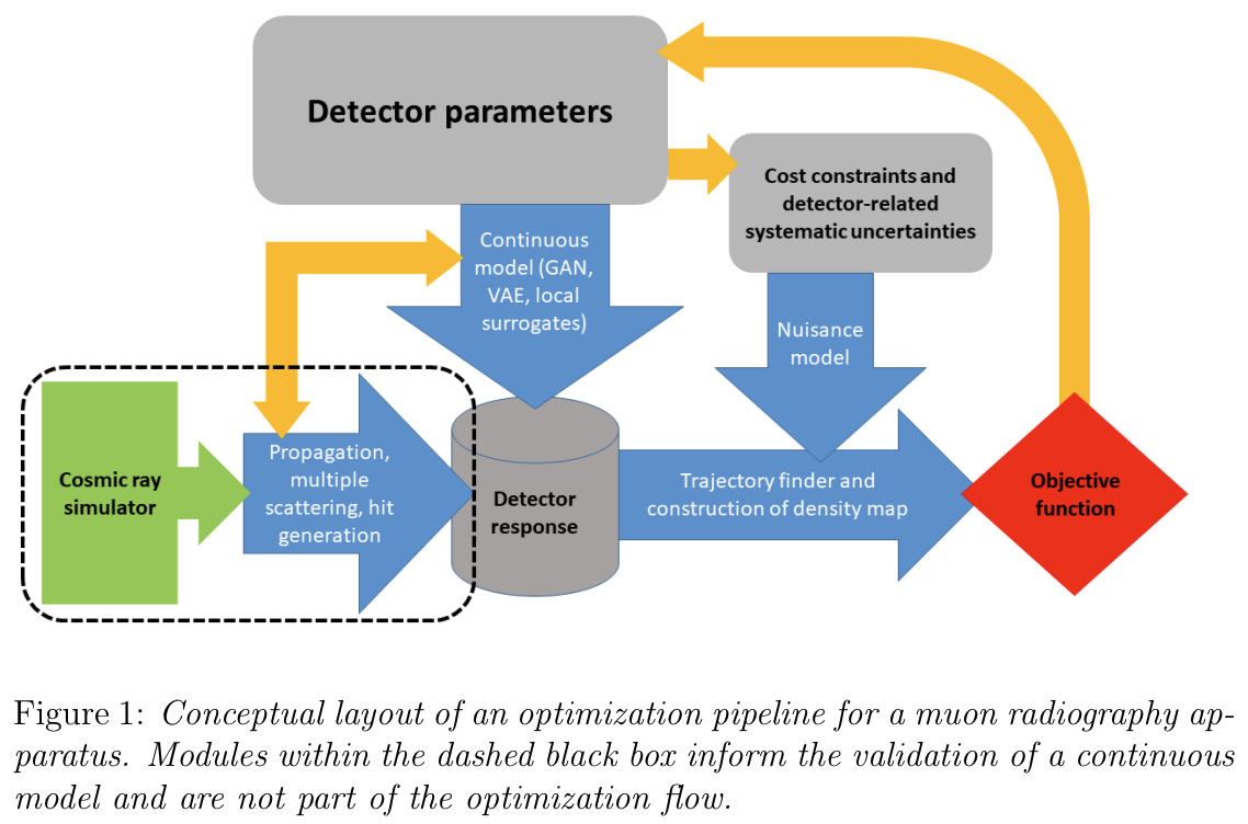
By careful construction of the simulation and inference chains, the final objective function can be differentiated with respect to the detector parameters, which can be updated just like those in a neural network. Some parts of the chain may need to be substituted for surrogate models, either to speed up optimisation, or to make them differentiable. The objective, here, can account for not only the performance (physics sensitivity, imaging accuracy, etc.) but also the budgets required to build the detector (which could be fiscal, heat generation, power consumption, space occupied, etc.).
Whilst other optimisation techniques exist (e.g. genetic algorithms and simulated annealing), a few of the advantages of differential optimisation are that:
-
The region of optimal solutions can be explored; as discussed in Mikhail Belkin’s (Halicioğlu Data Science Institute, UCSD) keynote talk, large systems are unlikely to converge to a single minima, but rather to a manifold of degenerate minima. By moving along these manifolds, we can sample designs which are expected to perform equally well, but might be more or less feasible to build. Similar to how Fast Geometric Ensembling (1, 2) produces multiple models from a single training.
-
Since parameters have physical meaning, and we know analytically how they affect the performance, design interpretation becomes much easier: e.g. “increasing the detector width improves the performance by a measurable rate”. Similarly, unintuitive changes can be identified and examined
The rich diagnostic feedback available, and the potential to have multiple designs, means that a framework built around differential optimisation could be invaluable as an assistive tool to detector optimisers. Of course we can never fully simulate all aspects of a detector design to the required detail, nor substitute the expert knowledge of detector designers; our aim is to provide tools to augment their workflow (like predictive text or driver assistance) and to better include notions of the final goal of the experiment. As an example of something similar to this, Auralee Edelen (SLAC) showed in her talk how ML-driven assistance tools could aid experts in tuning their machinery, reducing setup times from ~400 hours/year (~$12M), to about 7 hours/year.
Differential Optimisation in Action
So far this all sounds too good to be true, so the obvious questions are “Does it work? Can it be done?”.
In addition to the talks already mentioned, throughout the workshop we heard examples of how DP is being used for individual parts of experiments (e.g. final stage inference, data simulation, and reconstruction algorithms) in a wide variety of applications:
-
Topographical imaging and material ID: Volcanic eruption prediction, furnace calibration and damage detection, nuclear waste detection
-
Optimal signal inference under systematic uncertainties: INFERNO, Neos
-
Nuclear physics: detector calibration, data preprocessing, learning particle potentials
-
Neutrino physics: neutrinoless double-beta decay detection, reconstruction in Cherenkov detectors, track reconstruction and clustering
So the technology exists and is being used for reconstruction and inference. But what about in detector optimisation? We heard how IceCube and P-ONE were looking to use automated detector optimisation to help design their next generation of neutrino telescopes, so there’s definitely a demand for it. So how are we progressing on that front? For that, we had two presentations, both from MODE members.
Calorimeter optimisation
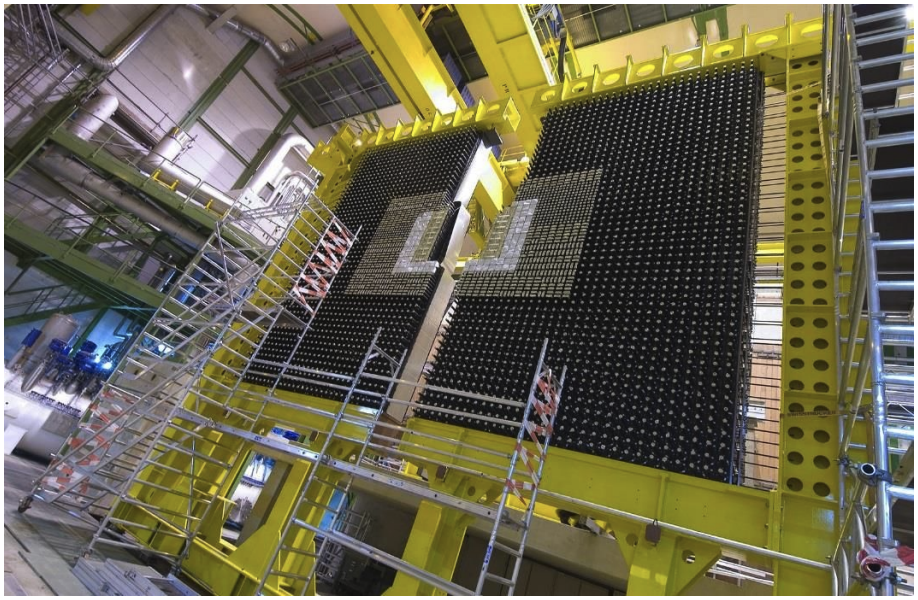
Alexey Boldyrev (MODE, Lambda-HSE) spoke on how he and his team were working on optimising the electromagnetic calorimeter (ECal) for the LHCb experiment. Pictured below, the ECal consists of an array of detection modules for measuring the particle showers produced by electromagnetic particles. A range of modules are available, each with varying performance and costs, so with future upgrades planned, the question is “How should a fixed budget be spent to gain maximum performance?”.
Their approach so far is to simulate the detector responses using Geant4 (an accurate, but non-differentiable detector simulator), reconstruct particles using a boosted decision tree (BDT) regressor (again, non-differentiable), and evaluate a performance metric. This process is relatively slow, and so in order to optimise the detector layout, they fit a Gaussian process model to the evaluated points. This surrogate model can then be used for Bayesian optimisation, in which regions of expected high-performance (exploitation), and regions of unknown performance (exploration) can be evaluated using the full simulation, and used to update the surrogate model.
Whilst this doesn’t yet make use of DP, it does show how automated design can be applied to complicated detectors. Their future plans include approximating the detector response with a differentiable model (GAN), and replacing the BDT with a neural network (again, differentiable), both of which will help move the study towards being able to leverage DP for optimisation.
Muon tomography optimisation
This workshop was a particularly special occasion for me, since I was able to show off a project I, and Dorigo, had been working on: TomOpt - a python framework for providing differential optimisation of detectors for muon tomography, using PyTorch as a backend. This is meant to be a first step into investigating the applicability of the fully differentiable pipeline we outlined in the MODE article (Figure 1). Muon tomography is a useful technique with a wide variety of applications (as was seen in prior presentations), but from an optimisation point of view, is comparatively simple. Given this, and the industry connections and experience within MODE, it seemed a good place to start testing our pipeline.
The aim of muon tomography is to infer characteristics of a volume of space (e.g. check the contents of shipping containers, to identify hazardous materials in sealed barrels, or to indicate area of damage in machinery). Muons are created when cosmic rays interact with the Earth atmosphere, and we can exploit their high penetration power to image volumes; by measuring their incoming and outgoing trajectories using detectors, we can infer what matter they interacted with, and where. The optimisation question is then “How should we configure the detectors to achieve optimal imaging precision for a given budget?”, and this is what TomOpt aims to help with.
The process consists of several stages:
-
Muons are generated by sampling random functions.
-
The muons pass through the incoming detectors, and record hits, which are differentiable with respect to the detector parameters we aim to optimise.
-
The muons pass through the hidden volume, and undergo scattering due to the varying density of material.
-
The muons pass through the outgoing detectors and record a second set of hits.
-
Muon trajectories are fitted to the incoming and outgoing hits, and are also then differentiable w.r.t. the detector parameters.
-
We use the trajectories to infer the densities of the hidden volume and pass the predictions to a loss function
-
The loss function contains two components:
-
The error of the predictions (how different the predictions are from the true values);
-
The cost of the detectors (computed at the current detector parameters).
-
-
This loss can then be differentiated w.r.t. the detector parameters, which can then be updated by gradient descent.
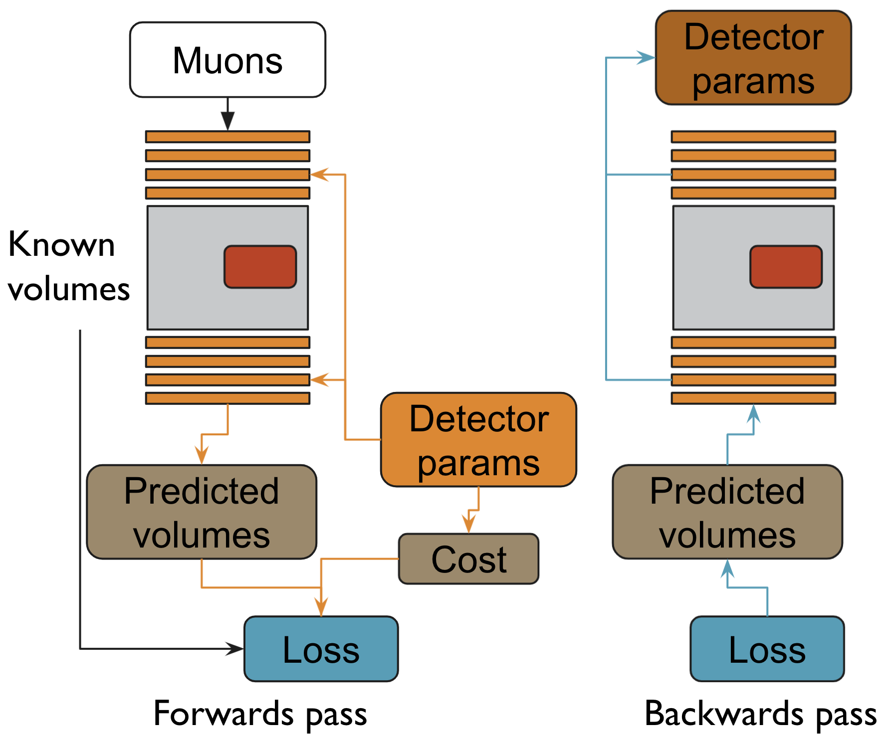
After a few rounds of such an optimisation process, we should arrive at a detector setup which is close to budget and provides good imaging. Currently, though, this is still very much in development, but we’re making progress!
Conclusion
This was the first workshop organised by the MODE collaboration and from the number of attendees (105, of which 39 were speakers), it is clear that there is both great interest and progress in the area of differentiable programming for experiment optimisation. There are even more talks than what I could include here, so I’d recommend checking the agenda. We should soon have recordings of the talks available, too. If any of this work sounds interesting and you are looking to work on similar topics, you may wish to consider contacting MODE to help coordinate efforts.