Remembering Protons: Memory maintenance systems for Agentic AI
Can particle-physics inspired algorithms improve memory maintenance in Agentic AI?
- Memory systems
- Memory maintenance
- Traditional approach
- What are memories, really?
- Sequential recombination for memory clustering?
- Importance weighting
- Anti-kt and generalised sequential recombination
- Conclusion

Memory systems
In Agentic AI systems, memory systems are a convenient way to adapt the system to the user, the particular system the user is working with, or to keep up to date with the latest information, conventions, software changes, etc. As the AI works through its usual tasks, it may encounter cases in which it lacks particular knowledge and has to learn it somehow (trial and error, user feedback, web searches, etc.), or finds that its most probable course of action disagrees with the user’s wishes or the current state of reality. Once the AI has course corrected, and learnt a better way to continue when faced with such cases, rather than having to repeat the same processes and mistakes later in the future, it can be more expedient to save this information as a memory, which can later be retrieved if the AI faces similar situations in the future.
Some examples:
- The agent tries to run commands in the user’s local system.
- The agent tries and fails.
- User tells the agent that it should be running the commands inside docker for this project.
- The agent tries again and succeeds. It saves this knowledge as a memory.
- The next day, the agent recalls the memory, and runs commands inside the docker container straight away.
- The agent tries to answer a question about the latest developments in a particular field, but it only has access to information up to 2024. It performs a web search, finds the relevant information, and saves it as a memory for future reference.
- The agent tries to use a particular software library, but it is not compatible with the current version of the user’s operating system. The agent learns that it needs to use an alternative library, and saves this information as a memory for future reference.
- The user has a particular preference for how the agent should format its responses. The agent learns this preference through interactions with the user and saves it as a memory to ensure that future responses are formatted according to the user’s preferences.
In a recent project, focussed on using agentic AI to build Magic: The Gathering decks, I recently introduced a memory system that allows the deck-construction agent to save information about specific cards that are available, strategies, card combinations, and the general state of the meta. This knowledge can only be learnt as the agent carries out its tasks, and examines the available cards (~7000) from different perspectives. It therefore becomes invaluable as the system is able to self-learn, and adapt as new cards are released and old ones retired.
Memory maintenance
Whilst they are beneficial, several potential issues can arise as memories begin to accumulate:
- Duplicate memories: Multiple memories contain highly overlapping information; they should be merged into a single memory.
- Obsolete memories: As the agent progresses, it may find information that is more useful than that currently contained in its memory collection; the new memory should replace the old one.
- Out of date information: As time goes by, some memories may become outdated and no longer relevant; they should be removed from the memory collection.
- Irrelevant memories: Some memories may have been accidentally saved because they were thought to be generally useful, but in actuality were so specific to a particular situation that they are not useful in other contexts; they should be removed from the memory collection.
- Conflicting memories: Some memories may contain conflicting information; this conflict should be resolved, or the specific circumstances in which each memory is relevant should be better clarified.
Eventually, it becomes necessary to perform maintenance on the accumulated memories, in order to address the listed issues. This could be as simple as automatically retiring old memories after a certain amount of time has passed since they were created. However, this can easily lead to loss of genuinely useful information. In my MTG Deck-Building system, my approach is to regularly run a dedicated agent over the memory collection. The agent is free to consider the benefits of each memory, both separately and together, and in the context of which cards are no longer in play due to retirement or bans. Finally, the agent outputs a refined collection of memories and the old memories are deleted.
The above description is actually a simplification: If a single agent were to consume all memories simultaneously, there is no guarantee it can scale well – in my system, a single pool of memories exist, which all user agents draw from and contribute to. As the number of users and memories grows, eventually, the memories will no longer fit into the context window of the LLM, and even before that, memory maintenance performance is likely to drop off well before the context limit is hit. Instead, what I actually do is to try to group similar memories together into clusters, and then run agents in parallel, once over each cluster. Each agent is still free to output as many new memories as it wants, but hopefully the clusters will be formed such that they contain one dominant kind of memory, with perhaps a few outliers. This allows the agent to consider all duplicate information at once and merge it to a single memory.
The topic that I will focus on in this post is how to best form these memory clusters.
Traditional approach
After some quick research, I found that a common approach to clustering memories is to use Hierarchical Density-Based Spatial Clustering of Applications with Noise (HDBSCAN). The basic premise of the algorithm is that it clusters points within regions of persistently high density, and can handle clusters of varying shapes and sizes, as well as noise (outliers). In our case, points are memories, and noise could be one-off memories that don’t belong to any particular clusters.
As for the coordinates for the points, we can use embedding models to project the text of the memory into an embedding space, where similar semantic concepts are naturally grouped together. Such an embedding should mean that similar memories appear naturally close together, thus becoming amenable to clustering.
In practicality, however, the density estimation directly in embedding spaces can lead to poor estimates, and so some form of dimensionality reduction is used to reduce the embedding space (~1024 dimensions) to something more manageable (2-3 dimensions). PCA, t-SNE, and UMAP are candidate algorithms. UMAP is often used for clustering-oriented workflows, while t-SNE can produce useful local neighbourhood structure, though distances and densities in t-SNE space may not be reliable.
Using some pseudodata data, let’s see the results of this approach. In the image below, both sub-images show the memories projected into 2D using UMAP. Each colour corresponds to a different cluster. The left sub-image shows the true class ID that the memories should be clustered to. The right sub-images shows the predicted cluster IDs after applying HDBSCAN. Points in dark blue (cluster ID “-1”) are memories that are determined to be noise, according to HDBSCAN. Ideally, memories coming from the same class should be clustered together.
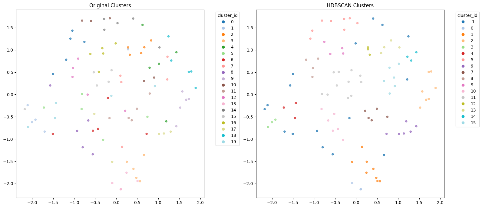
By eye, we can see that HDBSCAN does a good job of clustering points within the same spatial region, identifies outliers, and adapts for differently shaped clusters. We can also see that even at the UMAP level, however, some points belonging to the same class, but are positioned close to one another, making it hard for them to be clustered together. It is also hard to judge just how well the clustering process performs.
Both the dimensionality reduction algorithms, and HDBSCAN have a range of hyper-parameters, and what I want to do is to optimise these. But first I need to quantify what “performance” is.
Optimisation
In order to quantify what we mean by “performs” we need to introduce some metrics, that are representative of our task: We want to cluster similar memories together, such that an agent-swarm can output a reduced set of most representative memories. Given my budget, I’ll leave end-to-end metrics aside for now, and approximate this task to: We want to cluster similar memories together, such that each cluster contains a high proportion of true same-class memories, and the number of resulting memory clusters is not too high.
A variety of metrics are available to quantify clustering performance. I’ll examine several of them, but focus mostly on:
- B-cubed precision – The average of: Of the items placed in the same predicted cluster as memory i, how many truly belong with i?
- B-cubed recall – The average of: Of the items that truly belong with memory i, how many did the algorithm recover in its predicted cluster?
For my approximated task, I want to have a high recall, such that duplicate memories can be refined into a single memory, while controlling precision, to ensure that all memories are not turned into a single cluster. After an initial investigation to check metric ranges, I opted to maximise recall, subject to precision > 0.25.
For this research, I generated multiple pseudodata dataset based on possible MTG-related memories. Each memory is assigned a class ID, which represents the ideal cluster it should belong to. Optimisation is based on observing the average clustering performance over leave-one-out clusterings of the training data. Afterwards, the optimised hyper-parameters are tested on multiple validation datasets, to test generalisation.
Opting for a parametric, constrained, non-differentiable optimisation approach, I built a parameter space that covered the hyper-parameters of HDBSCAN, and a range of dimensionality reduction algorithms (None, PCA, t-SNE, UMAP), plus their associated hyper-parameters. Using Bayesian optimisation, I arrived at a set of hyper-parameters that performed well across several validation datasets, achieving an average performance of 0.62 B-cubed recall for 0.43 B-cubed precision, treating all noise predictions as a single cluster. UMAP was found to be the preferred dimensionality reduction algorithm, but interestingly, the optimal number of dimensions was found to be 1. The question is, can we do better than this?
What are memories, really?
I introduced memories as a concept that allows the AI system to learn, adapt, and record. When the system uses a memory it enters into the model’s context. We can suggest, then, that memories are instructions that should be present in the model’s context. But if that’s the case, why then can we end up with multiple memories carrying slightly different instructions? Because the memory creation mechanism itself is noisy – the agent generates memories in response to what it encounters, and may not perfectly understand the situation, or its nuances. The optimal way to deal with such situations (theory) are the instructions that should be given to the agent. However memories are not this, instead they are noisy observed approximations (experiment) of the true instructions.
As a high-energy particle-physicist I’ve encountered a similar phenomenon before, in the form of jets. The theory of quantum chromodynamics deals with quarks and gluons (partons) at a mathematical level, however colour-confinement means that such sub-atomic particles cannot be measured directly by experiment, such as those performed at the Large Hadron Collider at CERN – the partons instead hadronise long before they reach the scientific instruments designed to measure particle collisions. Instead what hits the detector is a collimated spray of particles and energy caused by the partons emitting new particles, radiating energy, recombining into colour-neutral particles, and finally decaying into the particles that we actually observe.
How, then, can we use particle colliders to test our theories if we cannot directly measure the particles that our theories are so dependent on? The key is to introduce the phenomenological concept of jets – cluster the energy deposits recorded by the detector, and treat them as approximations of the partons that they originated from. The image below (courtesy of ATLAS) shows an example of a jet constructed from a collision at the ATLAS detector at CERN. The blue and green cones represent the four jets that were reconstructed from the energy deposits in the detector.
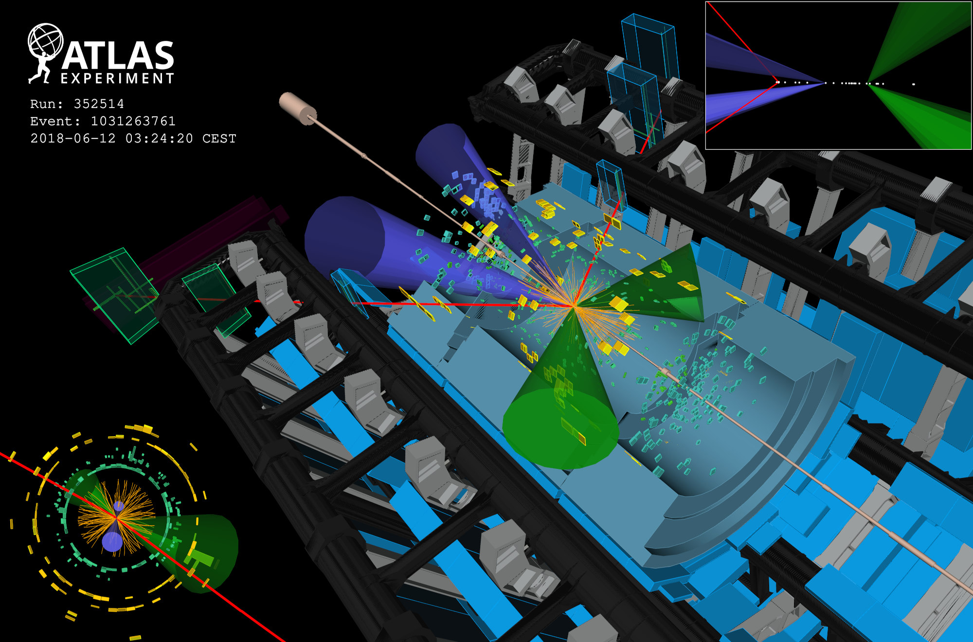
The type of algorithm used here is based on sequential recombination: energy deposits in the detector are iteratively recombined together, based on certain rules, until stop conditions are met. The recombination rules are based on factors such as separation between deposit pairs, and their energy. Sequential recombination algorithms are designed to be collinear safe and infrared safe. Basically this means that if a particle splits into two nearly parallel particles, then the algorithm should recombine them into a single jet. Similarly, if the particles radiate small amounts of energy, the resulting deposits should not significantly affect the reconstruction of the resulting jet, and should not seed jets of their own.
The term “recombine” is used here: the parton (theory) splits, radiates, and gradually scatters across a large area. We attempt to reconstruct it by recombining the resulting energy deposits.
Going back to memories, we can imagine a similar situation: the ideal instruction sentence can be reworded, split, translated, or otherwise perturbed many times, resulting in multiple observed memories, each of which ends up with some coordinate in our embedding space. This got me wondering whether a similar process of recombination can be used to cluster memories in order to approximate the (embedding of the) ideal instruction.
Because embeddings are non-injective, and because the ideal instruction is itself latent rather than observed, we should not expect to reconstruct a unique original instruction. But clustering around its approximate location may still be useful.
Sequential recombination for memory clustering?
The simplest sequential recombination algorithm is Cambridge/Aachen (C/A, [1997, 1999]). This defines a radius parameter R for the cut-off, and then iteratively combines points based on the closest pair, until all points are further than R away from each other.
Let’s extend this to an embedding-based clustering algorithm. We can work in the reduced-dimensional space (or the original space). Combining points means updating their coordinates to the pair’s mid-point. We can also remember that we have embedding vectors per point, and introduce a minimum threshold on the cosine similarity between the candidate pairs. The embedding vector of a combined pair can also be averaged, however we need to renormalise back to a unit-vector each time.
Performing a similar optimisation on this C/A-inspired algorithm, I found that it can achieve a better recall than HDBSCAN, at about the same precision level. C/A also compares favourably to HDBSCAN in terms of other metrics, too (for all metrics, higher is better).
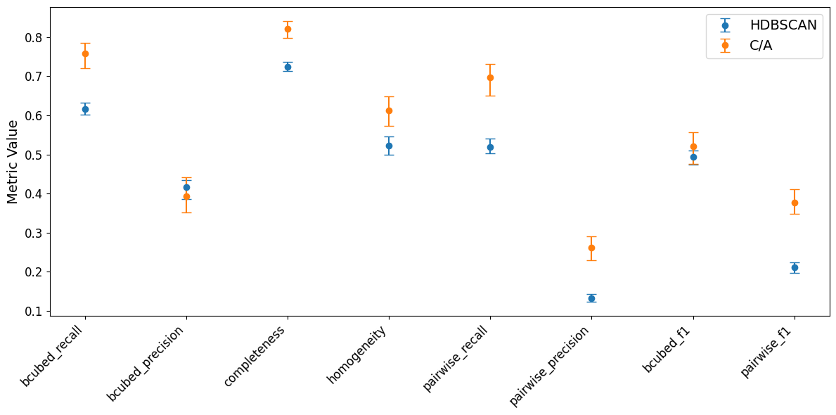
Optimisation of C/A resulted in using t-SNE for dimensionality reduction, with 2 dimensions. A very slight cut on cosine similarity of 0.03 was used, but likely not a significant factor and could be ignored.
Importance weighting
Let’s extend the memory system, now, and consider how not all memories may be equally important: some could only be important in very specific cases, others may be helpful, but not essential, and others could be so important that the system fails without them. An importance measure (weight) could be assigned to memories through a number of mechanisms, e.g. during creation, a sub-agent analyses the memory and assigns a predicted importance to it, or the importance could be inferred from the number of times the memory is retrieved. Assignment mechanism aside, the question I want to explore in the second half of this post is how the memory weights should affect clustering.
To begin, I’ll introduce weighted versions of the previous metrics, and analyse the performance of the previously optimised algorithms on weighted pseudodata.
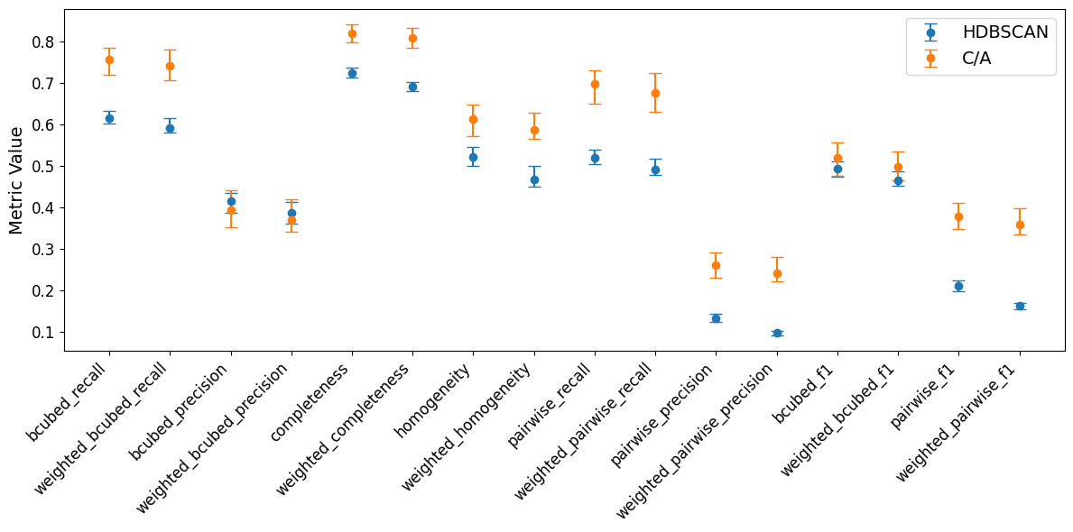
Whilst performance stays generally consistent between weighted and unweighted metric pairs, across the board we can see a very slight systematic underperformance on the weighted data. Certainly not catastrophic, but maybe we can try to better account for the importance during the optimisation and algorithm itself.
Weighted optimisation
A weighted version of HDBSCAN is probably possible: it computes point density across space, and a weighted version would involve changing the density computation to use point weights, rather than counts. However the library I use is highly optimised Numba code, and I don’t have the time to implement this myself, so I’ll leave this for another day. The best I can do for now, is simply to perform the optimisation considering the weighted metrics, rather than the unweighted ones.
For C/A, we can introduce a weighted version of the algorithm: the simple change to use weighted averages when recombining points and embedding vectors, such that the combined point and embedding is closer to the more important memory. When combining points, their importance weights are summed. Other aggregation rules are also possible, and could well be parameterised and optimised, but for now I’ll just use these.
For the purpose of optimisation, I initially scale all weights to be between 0 and 1.
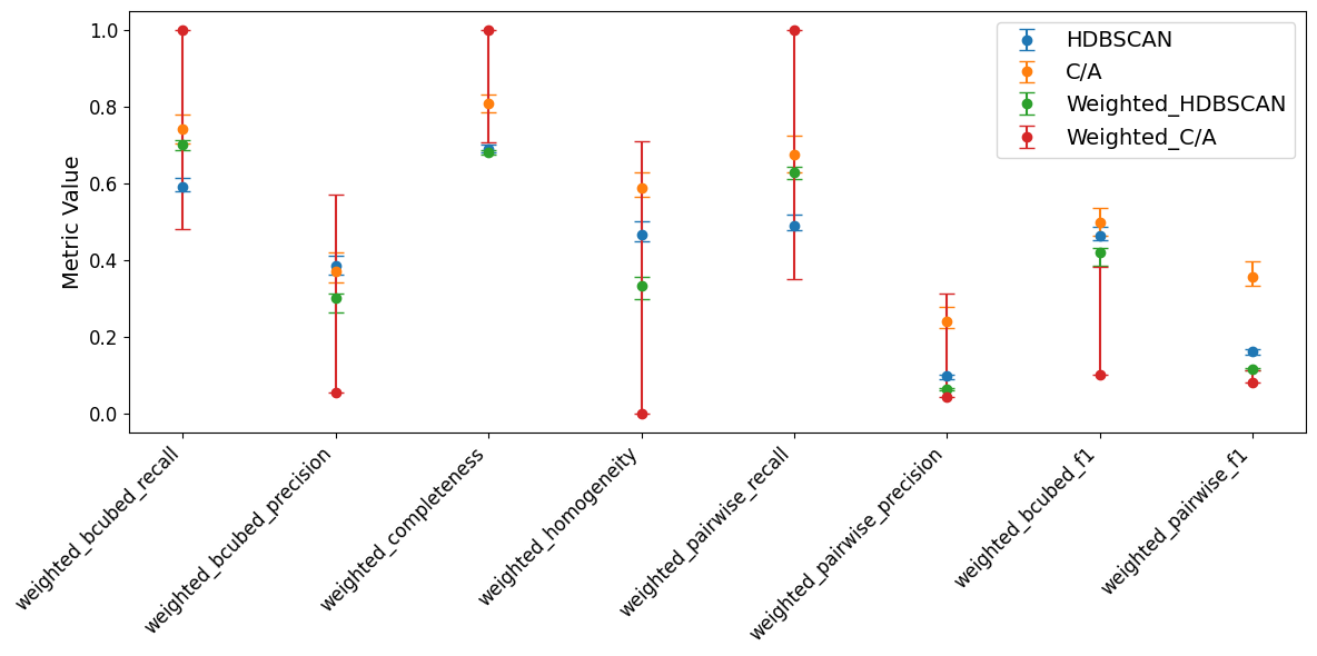
Alas, while the weighted optimisation of HDBSCAN results in a slight improvement on the weighted metrics, the weighted optimisation of C/A completely fails to generalise to validation data. Why is that?
Anti-kt and generalised sequential recombination
Thinking about the failure of our weighted version of C/A: the algorithm is only sensitive to the memory importances after the fact, i.e. importances are ignored when deciding which points to pair together. In particle physics, two other sequential recombination algorithms are used: kt [1993.1, 1993.2] and anti-kt [2008]. These are designed to not just consider the distance between points, but also their energy (or more strictly, transverse momentum, but let’s not get into that here).
They work on the basis of a generalised form of sequential recombination:
Where k_t is the transverse momentum of the point, delta_ij is the distance between points i and j, R is the radius parameter, and p is a parameter that defines the specific algorithm: p=1 for kt, p=0 for C/A, and p=-1 for anti-kt. The algorithm iteratively combines the pair of points with the smallest d_ij or removes the point with the smallest d_iB until all points are further than R away from each other. As p becomes smaller, the relative influence of the momentum/importance term grows. Distance still matters, but high-kt objects increasingly act as attractors that absorb nearby lower-kt objects.
The image below (source) compares the effect of different jet clustering algorithms, in terms of their resulting shapes.
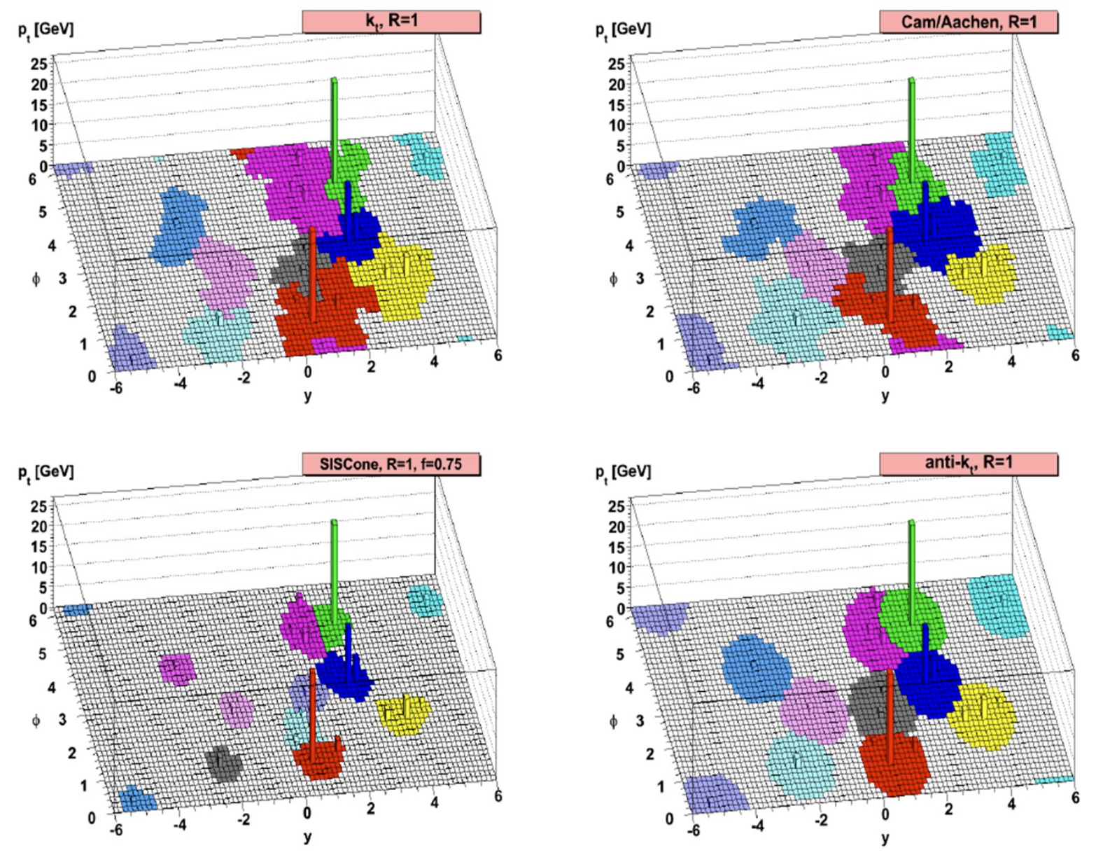
For our memory clustering case, we can use the memory importances as the transverse momentum. This allows the algorithm to also consider the importances when selecting combination candidates, rather than only being sensitive to it after the combination. For the memory-clustering variant, I deviate from the standard inclusive jet formulation by dropping the beam-distance removal step, d_iB. This deliberately biases the algorithm toward continued recombination and larger clusters, which better matches my maintenance-agent use case.
Let’s run optimisations using anti-kt (p=-1), and a general sequential recombination, in which p itself is an optimisable parameter.
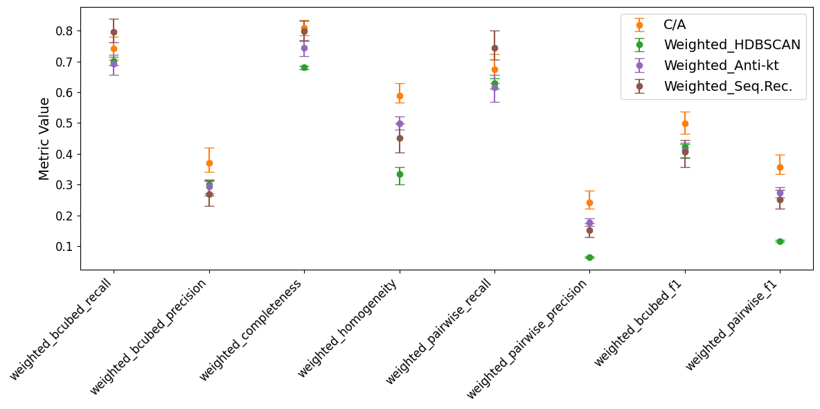
Allowing the importance weight to enter the candidate consideration allows both anti-kt and the generalised sequential recombination algorithms to generalise to validation data, without suffering the catastrophic failure seen in weighted C/A. Anti-kt itself appears to underperform, compared to unweighted C/A, however letting p float, allows the generalised sequential recombination algorithm to reach a very nice weighted B-cubed recall of 0.85, for a weighted B-cubed precision of 0.3. The optimal p value was found to be very low, at -1.69, which means that the algorithm is very sensitive to the memory importances, and less sensitive to their distance in the coordinate space (UMAP dim=3). A relatively large R parameter of 1.2 allows points to be quite far away from each other, and still be clustered together, however this is balanced by a moderate cosine similarity cut of 0.26.
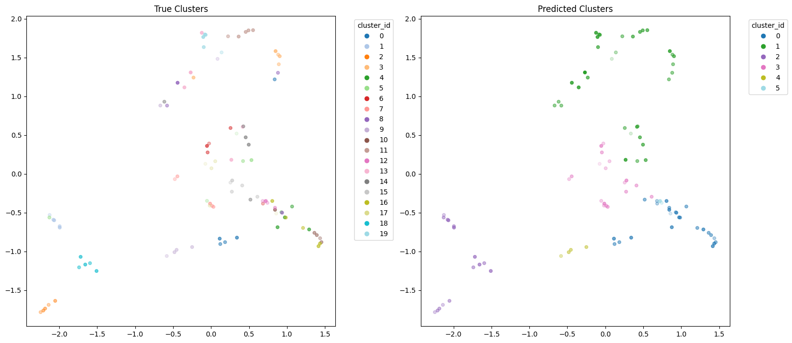
Below is an example clustering using the optimised sequential recombination algorithm. Certainly it is very heavy handed in terms of over clustering the data, reducing true number of classes from 20 down to 5 clusters. However, we can see that the true classes are somewhat intermingled, making perfect clustering very hard. Instead, we get what we asked for: close on 25% precision, with a very high recall. N.B. In the plot I show the first two dimensions of the 3D clustering space.
Conclusion
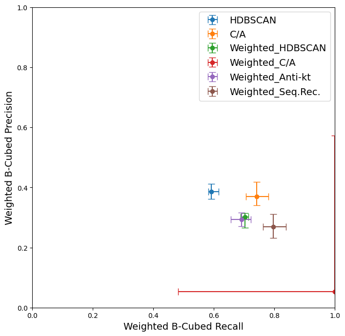
Comparing all of the optimised algorithms together, we can see that on these pseudo-data experiments, sequential recombination can improve over my HDBSCAN baseline, especially if importance weights are considered for the memories. Some form of dimensionality reduction is preferable, and in my testing I generally found that either t-SNE or UMAP performed well.
This said, I still have some doubts about the applicability of sequential recombination algorithms to memory clustering due to the sensitivity to distance: since I standardised and normalised the clustering space after dimensionality reduction, as more points/true classes are considered, the resulting clustering space becomes more densely occupied, and R-based clustering may become overly inclusive – it may be beneficial to scale R by some factor dependent on how densely occupied the clustering space is.
A further potential concern is that the optimal p value will also be sensitive to the range and scaling of the importance weights; non-linear scaling or larger ranges may require different p values to function optimally.
Additionally, it’s not yet clear to me how well the optimised algorithms will generalise to real memory data, which is likely to be much noisier than the pseudodata I used for testing. For now, what I may do is continue to use HDBSCAN for memory clustering, but also run the optimised sequential recombination algorithm in parallel, and save the results of how it would have acted. Later on I can then compare and see if it really does perform better, and if so, switch over to using it for memory maintenance.
Anyway, thanks for reading this far, and I hope you found it interesting! If you have any thoughts, suggestions, or questions, please do let me know.
P.S. I’ve uploaded the code I used for the sequential recombination algorithms here.